Go to Lecture 9 slides (Note: this explanation covers slide 23 onward)

Testing your design

When trying to design a new piece of software or hardware to solve a hard problem, inevitably you will ask yourself how to evaluate the performance of that new design compared to previous iterations. The answer : simulation. Simulating the new design in a controlled environment can give insights as to how well your solution performs. Below are two common ways of coming up with a simulation:

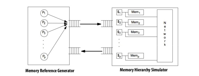
In execution driven simulation, you instrument a binary to record every memory load and store, and feed that data into your memory model.

In trace-driven execution, you want to record every memory store and load to be able to replay them later. This can be done by intrumenting the binary as before, or by running the program in a special simulator that will record the trace. For parallel programs, special care must me taken to preserve the timing of operations. [Show comments]

A word of warning: by definition, hard problems are difficult to solve. And, simulating a real system tends to be slow. Pragmatically, this means one of two things :

• A simulation that goes into lots of details will take forever to run;
• Conversely, a coarse grained simulation will be fast, but may not be accurate.

That last point, accuracy, is very important. It is very easy to inadvertently skew the results when attempting to make a simulation faster. When this happens, you end up with a useless, if fast, simulation that does not reflect how the system will behave at scale. This is covered in more details in the example below.

Scaling Down Challenges and Examples

There are various factors to consider when it comes to scaling down a program/simulation. These problems are mostly caused by the inherent links between the "scaleable" components of a program, and the difficulty in scaling down one component while keeping everything else constant. To illustrate this, here are some of the problems we can potentially run into.

1. Ratio of time spent on the different phases of a program could change with scaling
   • Barnes-Hut: Reducing the number of particles to run a smaller simulation reduces the density of particles in the grid, which in turn reduces the per-particle cost.
   • Assignment 2: Changing screen size but not the number of circles, will cause more time to be required for building per-block lists.
2. Removing contention by scaling down.
3. Changing communication to computation ratio by scaling down.
4. Changing one parameter may necessitate changes in other parameters.
   • Barnes-Hut: $n, \Theta, \Delta(t)$ are all related.

Barnes-Hut

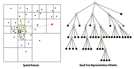
Barnes Hut is an algorithm for performing an n-body simulation, which a simulation for a group of celestial bodies whose positions in space change dynamically because of the gravitational force they exert on each other.

• Important parameters:
  • $\Theta$, threshold value for which given a body B and a region R, if s/d > Theta, where s is the width of R and d is the distance between R and B, then B can be approximated as a single body.
• Dividing the regions: Split space into quadrants recursively until each quadrant contains 1 or 0 bodies.

• Approach 1: Change $n$, the grid size.

  • We have to change $\Theta$, the threshold value, and $\Delta(t)$, the length of a time-step, accordingly.

• Approach 2: Change $T$, the total number of time-steps we run the simulation for.

  • There may be a larger proportion of time spent on setup and overhead costs.
  • Because of the reduction in the number of time-steps, the distribution of particles at the beginning and end are now different. This leads to a non-representative scaled-down simulation. One way to amend this is to take time-steps from the beginning and the end of the original simulation.

Assignment 2

A challenge of scaling down continues with the example from Assignment 2. For the purpose of debugging and testing we might want to perform render on smaller set of data, yet we want to preserve the traits of the original problem such as program behavior characteristics and scaling relationships between problem parameters as mentioned above. Thus, when scaling down an image there are multiple ways we can do apply.

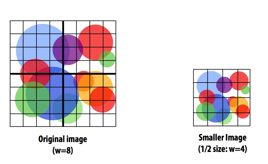
Approach 1 preserves other parameters such as number of circles, but scales down the image by reducing the number of pixels by a constant factor. However, a problem may rise as shrinking down image changes more parameters than expected. First, the circle distribution might have changed. Moreover, the work distribution to each thread block also changes as well. This can cause an issue by disturbing the workload of each thread in the block by assigning more circles that needs to be checked on each pixel or increasing the workload ratio of thread block as the dimension of the block remains the same.

As a result, rendering a shrunken image of pattern with size 256x256 results in 0.196ms in contrast to a full image of size 768x768 taking 0.840ms. This result shows that we cannot directly assume that the program would render image 9x faster just because the image has shrunken by 9 times. A possible reason for a slower speed up than expected is, as mentioned in the lecture comment, is due to increase in the number of circles per block.

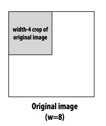
Approach 2 demonstrates a different approach of scaling down the problem size by cropping the image. This alternative solution preserves the workload of each block as the number of circles on the block remains the same. Therefore each pixel in the block will have same number of circles to check on as it did in the original problem. Note, however, that this analysis of Assignment 2 is very specific to the implementation of renderer. Thus, a different implementation might result in drastically different analysis of scaling down.

As the two examples beforehand have shown, scaling down a program is complicated due to the challenge of figuring out what parameter is the most relevant. Hence, it is important to know that these issues of scaling down also apply to the software developers when debugging or tuning the program on smaller machine with smaller dataset before running it on real machine with full dataset. This is because, when debugging, we often want to log the behavior of the program with printf statement. For example, as some might have experienced while debugging for assignment 2, using printf dramatically slows down a program. If rendering an image takes this long time, then it becomes inconvenient to debug the code with printfs on full dataset which would take dramatically longer time. Therefore, because the instrumentation slows down the code dramatically, we want to first debug and test our code with a smaller dataset. Moreover, as we will experience while we debug our code for assignment 3, using a real machine like Blacklight has long latency, as there is a long queue of people who are waiting to use it. Thus, it is more reasonable to debug and test the code on a smaller machine in Gates so that when you are given a chance, you can directly run your code on it.

The size of the problem/dataset matters not only to the programmers but also to the hardware architects. Since there are many parameters of the system such as the number of processors, cache size, cache line sizes, or memory bandwidth, simulating the performance of the hardware on each of the parameter is time consuming with full dataset. Therefore, it is more convenient to have smaller dataset to try on these parameters. To avoid trying all parameter space, another method of efficiently scaling down the problem for architectural simulation is deciding which parameter is relevant and prune the parameter space. The example on Figure 6. shows how to prune the cache size parameter space by analyzing the miss rate against the cache size, and by looking at the curve we can figure out at which point the cache size is adequate to avoid too high miss rate but also use space efficiently as highlighted by black dots on the graph.

Understanding the performance of parallel software

We want to analyze the part of the application that is limiting its performance(i.e. incurs most overhead, computationally most expensive etc). These parts include:

• Computation
• Memory Bandwidth
• Synchronization

We can measure the performance of parallel software by making use of high water marks, and use it as a "best-case scenario". To do this, we can utilize the following steps:

• How to establish a High Water Mark
  • Modify the code and observe the difference
  • Add non-memory instructions (An increase in runtime will indicate a computing bottleneck)
  • Substitute non-memory to memory instructions (An increase in runtime will indicate memory bottleneck)
  • Change all memory access to A[0] (This gives us an upper bound on the fastest speedup we can get by maximizing locality)
  • Remove all atomic operations, locks and thread synchronization (This gives us an upper bound on the fastest speedup we can get by minimizing synchronization)
• Record the best performance achieved

Questions

1. For barnes hut example, which simulator is more efficient between Trace-Driven Simulator and Execution-Driven Simulator?
2. When scaling down the assignment 2 from slide 28, we scale down the problem size in two different ways, yet both methods have only one thread block that renders the scaled down image assuming that 4 thread blocks were used to render full image. What is the difference in workload between the thread block in the shrinking image solution and the thread block in the cropping image solution? And how will that affect the performance of the threads in each block?
3. Explain the difference between Problem-constrained scaling and Memory-constrained scaling.
4. What can affect to the performance of parallel software other than Computation, Memory Bandwidth or Synchronization?