Introduction
Domain-specific programming systems play off of the idea of giving up generality and the ability to be used in many situations for high performance. A domain-specific system will put constraints on what a user can achieve in order to add extra guarantees on the data and optimize on those guarantees.
A great example of domain-specific programming systems are systems built for graph computation like GraphLab, Ligra and Green-Marl. There is a lot of inherent structure to a graph, like the fact that it consists of only vertices and edges. Since there is so much structure, a lot of assumptions can be made at the compiler level as well as the algorithmic level. The numerous pre-existing graph algorithms make algorithmic optimizations easy.
As a specific example of various optimizations that can be used, we will consider the specific case of implementing PageRank using GraphLab, Ligra and Green-Marl. An explanation of the PageRank algorithm can be found here. When observing the differences between the systems, one should consider which operations are made easy and at what cost? Why did the system architects pick those particular optimizations and what are their benefits?
GraphLab
GraphLab is an open-source project for describing iterative computation on graphs. It focuses on writing scalable machine learning algorithms on graphs using multicore processors and clusters. It is implemented as a C++ runtime.
The application state consists of the graph G, and read-only global data. The application defines data associated with each vertex and with each directed edge.
PageRank in GraphLab
PageRank is the graph algorithm at the base of the Google Search Engine. It forms a ranking of web pages based on the probability that a user randomly clicking through the web would land on a given page. The dampening factor $\alpha$ is the probability of leaving a vertex. In this section, we show how to implement PageRank in GraphLab
The language allows per-vertex update functions. These functions can read and write data associated with a vertex's neighborhood, where the neighborhood is defined as the vertex itself as well as adjacent (inbound and outbound) edges and vertices.
PageRank can be mathematically expressed as: $ R[i] = \frac{1-\alpha}{N} + \alpha \sum_{j \text{ links to } i} \frac{R[j]}{OutLinks[j]} $
Below is pseudo-code for PageRank in GraphLab, using GraphLab 1.0 style for simplicity.
PageRank_vertex_program(vertex i) {
  // (Gather) compute the sum of my neighbors rank
  double sum = 0;

  foreach(vertex j : in_neighbors(i)) {
    sum = sum + j.rank / num_out_neighbors(j);
  }

  // (Apply) Update my rank (i)
  double old_rank = i.rank;
  i.rank = (1-ALPHA)/num_vertices + ALPHA*sum
  i.change = fabs(i.rank - old_rank);
}
When the above code is run for a particular node, the pushed weight of each neighbor of the node is accumulated in sum, and ALPHA of this sum is given to the current node, and the rest is allocated for redistribution to neighbors.
i.change is used to determine whether the algorithm has converged, as can be seen in the following main program for PageRank:
// setup graph and vertex program here

double global_change;

while (!done) {
  signalall(); // execute program for all vertices
  global_change = reduce(change) // graphLab operation
  if (global_change < threshold)
}
In this way, we iterate until convergence.
The astute reader may realize that this implementation is inefficient. The majority of nodes in PageRank may converge in just a few rounds, and need not keep pushing weight around while waiting for other nodes to converge. This is particularly true for large graphs.
Consider the following GraphLab code, which fixes this problem:
PageRank_vertex_program(vertex i) {
  // (Gather) compute the sum of my neighbors rank
  double sum = 0;

  foreach(vertex j : in_neighbors(i)) {
    sum = sum + j.rank / num_out_neighbors(j);
  }

  // (Apply) Update my rank (i)
  i.old_rank = i.rank;
  i.rank = (1-ALPHA)/num_vertices + ALPHA*sum

  if(abs(i.old_rank - i.rank) > EPSILON) {
    foreach(vertex j : out_neighbors(i))
      signal(j); // Vertex i changed. neighboring vertices should be processed again.
  }
}
In the above code, signaling a vertex is similar to adding it to a work queue to have PageRank_vertex_program called on that vertex.
Granularity of Parallelism
GraphLab allows the program to specify the level of atomicity that GraphLab should provide. This determines the amount of parallelism. GraphLab offers the following levels:
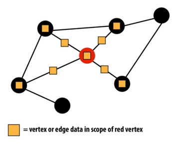
- Full Consistency: No other execution reads or writes to data in scope of v when the vertex program for v is running.
- Edge consistency: No other execution reads or writes to data in v or in edges adjacent to v.
- Vertex consistency: No other execution reads or writes to data in v or in vertices adjacent to v.
Job Scheduling Order
The work scheduling policy can be changed by the programmer between one of the following:
- Synchronous: Update all vertices simultaneously, meaning that each vertex does not see updates from program execution on other vertices in the same round.
- Round-robin: Vertex programs will observe the most recent updates
- Graph Coloring: We color the graph to split it into n independent sets, and execute on each of these sets in parallel.
- Dynamic: Based on new work created by signal
Note that a combination of the consistency policy and the scheduling policy determine program correctness. For example, with edge consistency, a program may be correct with any scheduler. With a graph coloring scheduler, however, the program can only be correct with vertex consistency.
It is important to realize that many graph alogirthms make assumptions about the schedule in which nodes are processed.
Ligra
Ligra is a lightweight parallel graph algorithms framework developed here at CMU. The framework is designed for shared-memory machines, presenting noteworthy advantages and disadvantages when compared to distributed architectures: Graph size is limited by the amount of memory one machine can hold (although this is very large these days) Synchonization is much more simple. CAS operations are sufficient to avoid most undefined behaviors from data races. Performance is not limited by communication times (network latency, etc.), reducing the amount of performance reasoning a programmer must do.
Programming in Ligra is very simple. Here are the important constructs:
CAS(loc, oldVal, newVal) atomically updates the contents of memory addess loc to newVal and returns true if the current contents are equal to oldVal, and returns false otherwise, without making any modification
SIZE (U : vertexSubset) computes the size of U
EDGEMAP(G : graph, U : vertexSubset, F : (vertex*vertex) -> bool, C : vertex -> bool) : vertexSubset
Applies F to all edges in $E_a = {(u, v) \in E | u \in U ^ C(v) = true}$
Returns the vertexSubset ${v | (u, v) \in E_a ^ F(u, v) = true}$
VERTEXMAP(U : vertexSubset, F : vertex -> bool) : vertexSubset
Applies F to every vertex in U.
Returns ${u \in U | F(u) = true}$
Implementing pagerank in Ligra is also very simple:
pcurr = {1/V,..., 1/V}
pnext = {0.0, ..., 0.0}
diff = {}
procedure PRUPDATE(s, d)
  ATOMICINCREMENT(&pnext;[d], pcurr[s]/(deg+(s))
  return 1

procedure PRLOCALCOMPUTE(i)
  p_next[i] = ($\alpha$ * p_next[i]) + 1 + (1-y)/|V|
  diff[i] = |p_next[i] - pcurr[i]|
  p_curr[i] = 0:0
  return 1

procedure PAGERANK(G, y, e)
  Frontier = {0, ..., |V| - 1}
  error = \infty
  while (error > e) do
    Frontier = EDGEMAP(G, Frontier, PRUPDATE, C_true)
    Frontier = VERTEXMAP(Frontier, PRLOCALCOMPUTE)
    error = sum of diff entries
    SWAP(p_curr, p_next)
  return p_curr
Ligra's data parallel model of mapping functions over edge and vertex sets makes graph traversal and mutation algorithms easy to write and analyze.
Green-Marl
(source: http://ppl.stanford.edu/papers/asplos12_hong.pdf)
Green-Marl is a DSL focused on exploiting data-level parallelism inherent in graph analysis. It allows the user to define their algorithms in an intuitive way, then compiles that code into an optimized parallel implementation in C++. This compiled code is written using OpenMP for conciseness.
Scope of the Language
As is typical of DSLs, Green-Marl is designed for certain operations or analyses of graphs. These are 1. Computing a scalar value from a graph and a corresponding set of properties (e.g. conductance of a sub-graph) 2. Computing a new property from a graph and a corresponding set of properties (e.g. pagerank) 3. Selecting a subgraph of interest (e.g. strongly-connected components) Note that properties are defined as a mapping from a node or edge to some data value.
To be optimized for these types of analysis, Green-Marl makes certain assumptions: 1. The graph cannot be modified during analysis (properties can be created and modified) 2. There are no aliases between graph instances nor graph properties. These assumptions allow the user to construct the graph in any manner he or she wishes, while allowing Green-Marl to focus only on analysing it.
Parallelism
The simplest way for a user to denote parallel computation in no particular order over a set of elements is by using a Foreach statement. Similar to OpenMP, this is achieved by forking the process once for each element, then synchronizing and joining just before the instruction after the Foreach. The following Green-Marl code shows nested parallel iteration:
Int sum=0;
Foreach(s: G.Nodes) {
  Int p_sum = u.A;
  Foreach(t: s.Nbrs) { // t : neighbors of s
    p_sum *= t.B;
  } // Sync
  sum += p_sum;
} // Sync
Int y = sum / 2;
Note that in Green-Marl, local variables are private to the current iteration step, but are shared in any parallel region in the same scope as that variable. For example, p_sum in line 5 is private and not shared between instances of the loop defined in line 2, but is shared between instances of the loop defined in line 4.
Memory Consistency
Memory consistency in Green-Marl is similar to the model in OpenMP:
- A write to a shared variable is not guaranteed to be visible to concurrent iteration steps in the same scope.
- A write to a shared variable is guaranteed to be visible to later statements in the same iteration step, unless a write to that shared variable from a concurrent iteration step becomes visible before that statement
- A write to a shared variable becomes visible at the end of a parallel iteration. If multiple concurrent iteration steps wrote to the same variable, only one write is chosen non-deterministically
- Each write, and each operation on a collection (e.g. adding an item to a set) is atomic
An example of a Green-Marl program that suffers from data-races follows:
Foreach(s:G.Nodes)
  Foreach(t:s.OutNbrs)
    t.A = // write-write conflict
      t.A + s.B; // read-write conflict
Line 3 is a W-W conflict because multiple s-iterations (loop iterations from line 1) can write to the same t node. Line 4 is a R-W conflict for the same reason.
Because of the narrow nature of DSLs, Green-Marl's compiler is able to identify such data-races at compile time and notify the user. By doing this, Green-Marl prevents the user from writing algorithms that communicate over concurrent iteration steps.
PageRank
What follows is an implementation of PageRank in Green-Marl
Procedure PageRank(G: Graph, e,d: Double, max_iter: Int, PR: Node_Prop<Double>(G)) {
Double diff =0;     // Initialization
Int cnt = 0;
Double N = G.NumNodes();
G.PR = 1 / N;

Do {       // Main Iteration.
  diff = 0.0;
  Foreach (t: G.Nodes) {    // Compute PR from neighbors current PR.
    Double val = (1-d) / N +
      d* Sum(w: t.InNbrs) (w.OutDegree()>0) {w.PR / w.OutDegree()};
    t.PR <= val @ t;    // Modification of PR will be visible after t-loop.
    diff += | val - t.PR |;    // Accumulate difference (t.PR is still old value)
  }
  cnt++;      // ++ is a syntactic sugar.
} While ((diff > e) && (cnt < max_iter));  // Iterate for max num steps or differe
The following figure shows the speed-up of a Green-Marl implementation of PageRank on graphs with 32 million nodes and 256 million edges. Performance was measured on a commodity server-class machine, which has two sockets with an Intel Xeon X5550, each with 4 cores and 2 hardware threads per core.
Questions
- What are the differences in optimizations between systems?
- How does each optimization affect the computational intensity of PageRank?
- Can you think of a situation (on graphs) for which each system would be a poor choice?