Here is some rough pseudocode for the modified algorithm. Note that this algorithm does not compute the same result as the original program given on slide 25, but it is still is a valid iterative solver. It is also much easier to parallelize.
 while (!done):
   diff = 0;
   for each red cell (i,j) IN PARALLEL:
     float old = A[i,j];
     # computing element A[i,j] depends only on itself and on
     # the surrounding black cells
     A[i,j] = 0.2f * (A[i-1,j] + A[i,j] + A[i+1,j] + A[i,j-1] + A[i,j+1]);
     diff += fabs(A[i,j] - old);

   for each black cell (i,j) IN PARALLEL:
     float old = A[i,j];
     # computing element A[i,j] depends only on itself and on
     # the surrounding red cells
     A[i,j] = 0.2f * (A[i-1,j] + A[i,j] + A[i+1,j] + A[i,j-1] + A[i,j+1]);
     diff += fabs(A[i,j] - old);

   check for convergence here ...
mperron
Would it also be valid to double the space required to ensure each cell's calculation is independent? That is, calculate the value for a cell, save it to a new matrix, repeat for all cells, then work from the new matrix until it converges? This could then be repeated by reading from one matrix and saving to the other, then swapping. This way, each cell only has dependencies in another matrix and will not collide as long as all workers wait for completion of an entire matrix before continuing.
Is this a valid approach?
Araina
@mperron, I think your answer can be an approach but may receive some efficiency loss from memory access of another matrix.
stl
@mperron, I think while your approach would work if our goal was just to ensure independence, it would end up producing a different answer than what would be given by the Gauss-Seidel method which is what we're simulating here. After reading a little about Gauss-Seidel on the Wikipedia page it seems like the algorithm is written with the knowledge that as you iterate through the matrix, neighboring values on the top and left will have already changed. This overwriting property is a key part of the algorithm producing its final answer and is also what allows the algorithm to be more space efficient because it can compute its answer and only have to allocate space for one matrix rather than two.
jpd
@mperron While that would be valid (since it's an approximation anyway), I don't think you'd actually gain much performance, since you lose the locality benefit of the computation that this model has (2 separate arrays could be very far apart in memory). It wouldn't change the convergence properties much (at least in most cases), and it would probably converge at about the same rate to the same approximate value.
maxdecmeridius
How is this the same as the previous program? Aren't the red cells at the bottom right still dependent on the changed black cells around it, which are dependent on the red cells to the top and left of it?
xx420y0los4wGxx
@maxdecmeridius
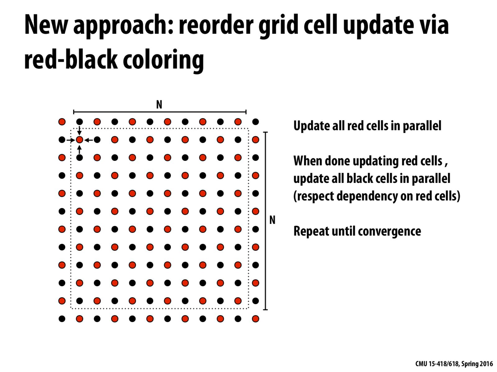
The program updates all the red spots (and black spots) in parallel. This means that on an individual iteration there is no guarantee (and most likely won't be) that the red dot will have the correct answer set in the matrix. We simply continue doing this until the algorithm converges. This results in better parallelism due to the number of dots that are being computed at once versus sometimes having larger diagonals and also the lack of dependencies.
Although to me this raises the question on the number of iterations this will take for the algorithm to converge and if in the worst case this would be better than a worse case of the previous algorithm.
enuitt
It is pretty tricky to compare this algorithm to the previous diagonal algorithm as they offer different results. This red-black version seems to calculate the entire board once very 2 iterations, whereas the diagonal algorithm seems to calculate the entire board after running through all the diagonals ( about length_of_board x 2 iterations). Hence this version seems to be much more efficient. Is this even a valid way of comparing the 2 algorithms?
And can there be cases where one algorithm converges while they other does not?
traveling_saleswoman
Perhaps one way you could see compare the two algorithms is by seeing 1. which one converges for more inputs, 2. which one converges faster, and 3. which solution leads to a better overall performance in the context of the whole application. As we saw in Lecture 8, this grid solver is used in ocean current simulation. You could compare the algorithms by seeing which version produces a more accurate simulation compared to the real outcome.
tdecker
Does this type of technique scale when you have a more complex graph. This example could be make into a bipartite graph. What if the graph was at minimum 3 colors or 4 colors.
Here is some rough pseudocode for the modified algorithm. Note that this algorithm does not compute the same result as the original program given on slide 25, but it is still is a valid iterative solver. It is also much easier to parallelize.
Would it also be valid to double the space required to ensure each cell's calculation is independent? That is, calculate the value for a cell, save it to a new matrix, repeat for all cells, then work from the new matrix until it converges? This could then be repeated by reading from one matrix and saving to the other, then swapping. This way, each cell only has dependencies in another matrix and will not collide as long as all workers wait for completion of an entire matrix before continuing.
Is this a valid approach?
@mperron, I think your answer can be an approach but may receive some efficiency loss from memory access of another matrix.
@mperron, I think while your approach would work if our goal was just to ensure independence, it would end up producing a different answer than what would be given by the Gauss-Seidel method which is what we're simulating here. After reading a little about Gauss-Seidel on the Wikipedia page it seems like the algorithm is written with the knowledge that as you iterate through the matrix, neighboring values on the top and left will have already changed. This overwriting property is a key part of the algorithm producing its final answer and is also what allows the algorithm to be more space efficient because it can compute its answer and only have to allocate space for one matrix rather than two.
@mperron While that would be valid (since it's an approximation anyway), I don't think you'd actually gain much performance, since you lose the locality benefit of the computation that this model has (2 separate arrays could be very far apart in memory). It wouldn't change the convergence properties much (at least in most cases), and it would probably converge at about the same rate to the same approximate value.
How is this the same as the previous program? Aren't the red cells at the bottom right still dependent on the changed black cells around it, which are dependent on the red cells to the top and left of it?
@maxdecmeridius
The program updates all the red spots (and black spots) in parallel. This means that on an individual iteration there is no guarantee (and most likely won't be) that the red dot will have the correct answer set in the matrix. We simply continue doing this until the algorithm converges. This results in better parallelism due to the number of dots that are being computed at once versus sometimes having larger diagonals and also the lack of dependencies.
Although to me this raises the question on the number of iterations this will take for the algorithm to converge and if in the worst case this would be better than a worse case of the previous algorithm.
It is pretty tricky to compare this algorithm to the previous diagonal algorithm as they offer different results. This red-black version seems to calculate the entire board once very 2 iterations, whereas the diagonal algorithm seems to calculate the entire board after running through all the diagonals ( about length_of_board x 2 iterations). Hence this version seems to be much more efficient. Is this even a valid way of comparing the 2 algorithms?
And can there be cases where one algorithm converges while they other does not?
Perhaps one way you could see compare the two algorithms is by seeing 1. which one converges for more inputs, 2. which one converges faster, and 3. which solution leads to a better overall performance in the context of the whole application. As we saw in Lecture 8, this grid solver is used in ocean current simulation. You could compare the algorithms by seeing which version produces a more accurate simulation compared to the real outcome.
Does this type of technique scale when you have a more complex graph. This example could be make into a bipartite graph. What if the graph was at minimum 3 colors or 4 colors.