Question: Can someone summarize how the partitioning of source RDDs can affect the cost of the join transformation? How does your answer motivate the partitionBy operation described on the next slide?
ghawk
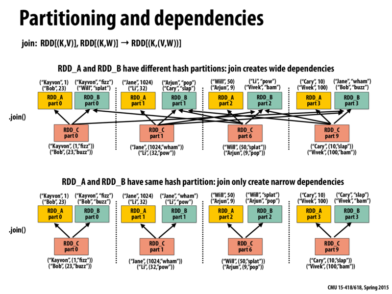
In the first case on top of the slide, the data is not partitioned consistently across the two RDDs A and B. For example, the key "Bob" appears in RDD_A in part0, but the same key appears in part3 for RDD_B. A join operation would hence require a network communication operation, where the key Bob from RDD_B's part3 partition is moved to the node where part0 resides. This would be fairly expensive as it can lead to $n^2$ network messages, for a join operation on $n$ keys.
We can instead partition the two RDDs, using the same partitioner on the keys of the RDDs. This will ensure that data of the two RDDs with same keys will reside in the same partition (or node). This will help avoiding the network communication overhead, and speed up the join operations by reducing communication.
This approach is very similar to the HashPartitioner used in the next slide, as the next slide also uses the same partitioner for the partitionBy() function for both the RDDs.
Kapteyn
In both cases on this slide it seems like RDD_C is inheriting the partitioning rule of RDD_A.
The code on the next slide specifies the partitioning rule for "ClientViewPartitioned" and "MobileViewPartitioned" which get joined into "joined". But no where does it specify the partitioning rule to use for the joined RDD.
In the case where the two RDDs getting joined share the same partitioning, it makes sense for the joined RDD to share the same partitioning, but in the top case on this slide, where the two RDDs getting joined do not share the same partitioning, how does Spark decide which partitioning rule to use? That of RDD_A or RDD_B?
Kapteyn
Actually I just realized that since you're calling RDD_A.join(RRD_B) you would use the partitioning rule of the caller.
Question: Can someone summarize how the partitioning of source RDDs can affect the cost of the
jointransformation? How does your answer motivate thepartitionByoperation described on the next slide?In the first case on top of the slide, the data is not partitioned consistently across the two RDDs A and B. For example, the key "Bob" appears in RDD_A in part0, but the same key appears in part3 for RDD_B. A join operation would hence require a network communication operation, where the key Bob from RDD_B's part3 partition is moved to the node where part0 resides. This would be fairly expensive as it can lead to $n^2$ network messages, for a join operation on $n$ keys.
We can instead partition the two RDDs, using the same partitioner on the keys of the RDDs. This will ensure that data of the two RDDs with same keys will reside in the same partition (or node). This will help avoiding the network communication overhead, and speed up the join operations by reducing communication.
This approach is very similar to the HashPartitioner used in the next slide, as the next slide also uses the same partitioner for the partitionBy() function for both the RDDs.
In both cases on this slide it seems like RDD_C is inheriting the partitioning rule of RDD_A.
The code on the next slide specifies the partitioning rule for "ClientViewPartitioned" and "MobileViewPartitioned" which get joined into "joined". But no where does it specify the partitioning rule to use for the joined RDD.
In the case where the two RDDs getting joined share the same partitioning, it makes sense for the joined RDD to share the same partitioning, but in the top case on this slide, where the two RDDs getting joined do not share the same partitioning, how does Spark decide which partitioning rule to use? That of RDD_A or RDD_B?
Actually I just realized that since you're calling RDD_A.join(RRD_B) you would use the partitioning rule of the caller.