


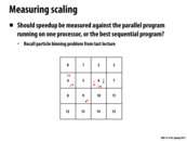

The point to be made here is that testing the parallel version of an algorithm against itself on 1-core vs many-cores can be misleading in that the parallel version on 1-core is nowhere near as fast as an optimized sequential version of the algorithm on 1-core.
This comment was marked helpful 0 times.

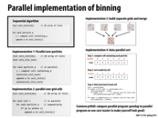
The different implementations also display the importance of our performance metric. For example, if our goal was to minimize contention, we would choose implementation 4. But, this implementation also does a lot more work, so if we wanted to instead have less work, we might choose implementation 3 (which has a larger contention problem).
This comment was marked helpful 0 times.

Usually an optimized sequential implementation is most efficient in the amount of work it is doing, although the parallel version of an algorithm may still be faster. And the reason here is that the parallel version achieves better parallelism (it does more work at once) which makes up for the more work it needs to do. And the more cores the machine has the algorithm can achieve greater speedup. Therefore, comparing parallel program speedup to parallel program on one core doesn't reveal the true result.
This comment was marked helpful 0 times.


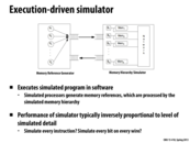
This graph shows how adding more processors does not always mean we will observe a speedup. When the problem size is too small, we may actually see a decrease in speed because communication costs outweigh the benefit of parallel computation.
Processor designers need to ensure that their allows for scaling down the number of processors used.
This comment was marked helpful 0 times.


Not every problem is worth trying to parallelize on many cores. If the problem is too small, the excessive overhead in communication makes it so that the performance gains are effectively moot and in some cases, can actually hurt performance.
This comment was marked helpful 0 times.
This doesn't truly reflect the usage of the 32-processor machine when the problem size is small enough. The ratio between by time consumed by communication and computation can vary a lot due to the size of the problem as well as the number of processors in the machine.
This comment was marked helpful 0 times.
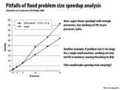

The ideal speedup has a slope of 1. Every time we add a processor, we expect the best time we can accomplish is the number of processors we currently have, multiplied by the best time we can achieve in single core execution. This isn't always the case, however, which leads to a speedup that is better than the ideal, called super-linear speedup. Contributing factors that can lead to a super-linear speedup involve utilization of the cache. Every time we add a processor (assuming each new core comes with its own L1 cache), the amount of aggregate L1 cache present in the system increases. The program's working set might be too large to fit in a single core's cache. However, when splitting the work up among many processors, the working set can be split up into chunks that can potentially be small enough to fit into each core's cache. As a result, execution of each core involves fewer cache misses than execution on a single core.
In the graph, we can see that between 8 and 16 processors, the working sets are likely split up enough that the data can be cached, thus causing the graph to become non-linear.
This comment was marked helpful 0 times.

There was a question in class about what the "ideal" line measures, and is it "ideal enough" because it doesn't make sense the speedup to be more than ideal. Basically, the ideal speedup line assumes that everything else about the machine will scale as we increase the number of processors. As @max mentioned, the number of cache misses doesn't necessarily do that (it actually goes down).
In general, I understand what the line is trying to communicate, but I think ideal is a bad name for it. Theoretical speedup might be a better name. Sort of analagous to inherent communication and artifactual communication, the line doesn't take into account the interaction between the application and the system.
This comment was marked helpful 0 times.

@Incanam: Good comment, but I'm not sure what you meant by "everything else about the machine will scale as we increase the number of processors". How I'd say is this: The "ideal" line on the graph corresponds to an intuitive notion of the speedup you'd expect to observe if the application was perfectly parallelized onto N processors. That is, in theory (not considering any low-level details of the system's implementation) if you took a program and perfectly distributed its work to N cores (perfect workload balance, no overhead of communication, synchronization, etc.), it is logical to expect to speed up execution by a factor of N.
This graph shows that in practice, sometimes you might observe a greater than N speedup. In this case, the reason is the caching behavior that @max and @Incanam have nicely explained above. Of course, there might be other reasons for a super-linear speedup as well.
Question: Many of you have observed a superlinear speedup for certain configurations on Assignment 3. This superlinear speedup is not due to caching behavior. What might it be?
This comment was marked helpful 0 times.

One possible reason is pruning. While doing DFS for WSP, shorter path found may cause more pruning and less calculation in later searching. For example, in shared memory model, if there exists a shortest path beginning with 2, and we do the two branches beginning with 1 and 2 simultaneously? the shortest path may reduce workload in the first branch, thus reduce total workload.
This comment was marked helpful 2 times.


As the past few slides have demonstrated, showing scaling of a program as a function of the number of cores on the same input can give misleading information about the scalability of a program. Therefore, it might be important to put thought into the input being used for timings. It may be possible to find a "middle ground" input that isn't strongly affected by the issues for too small or large problems listed above. Alternatively, showing the scaling for multiple inputs may be appropriate.
In other cases, it doesn't really make sense to be comparing the same input size in the first place. For example, the 258x258 ocean sim example may finishes pretty quickly with 8 processors, so I wouldn't be terribly concerned with its performance on 64 processors, since I can just run it on the 8 processor system.
This comment was marked helpful 1 times.

The trick used here is that computing capacity doesn't indicate directly the speed of the program due to the complicated hardware context. One reason is that other related hardware may change in amount or in structure, as cache size in the previous slide. The other one is that the increase/decrease of computing capacity may change infrastructure, e.g., from single core to multiple cores. So it is always too naive to judge by computing capacity only.
An interesting way to observe it is that to give the rate of speedup to each instruction. Data operation usually has negative rate, while computation operation has positive rate. You may cross product the proportion of different operations and speedup rate to estimate the ideal speedup. Normally, if data operations claim the most part of the program, we can always expect the great speedup.
This comment was marked helpful 0 times.


I understand the point of scaling up programs. However, what is the point of scaling down programs? It seems that when you write programs, you program according to how many processors you have. Why would you want to reduce that?
This comment was marked helpful 0 times.

@akashr I don't think you always know exactly how many processors your program will be run on. As the last bullet point mentions, CUDA is designed to work on both high-end and low-end GPUs. If you publicly released CUDA code, for example, people with both high-end and low-end GPUs could be running your code. So if you test and optimize your code on a GTX 680, you would probably also want to see how it scales down to a GTX 650 which has a lot less processors than the 680 since you will very likely have people with low-end GPUs trying to run your code.
This comment was marked helpful 2 times.

Question: In the ocean, isnt T/dt really one parameter, not two independent ones?
This comment was marked helpful 0 times.
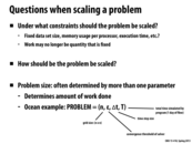
In the slide, dt is the amount of "simulated" time between two time physics time steps. T is meant to be the total duration of the physics simulation (careful: it's the simulated time, not the wall-clock time to actually run the simulation on a machine), so the total number of time steps is T/dT. An alternative, but equally expressive two-parameter set up would be dt and num_timesteps.
You need two parameters because num_timesteps time steps each of length dt is a different simulation than the same number of time steps, but with double the time (increased dT) per time step.
This comment was marked helpful 0 times.


Question: what would be a good example of user-oriented scaling?
This comment was marked helpful 0 times.
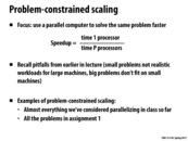
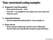
For each of the resource-oriented scaling, one variable is fixed, and the remaining variables are used to determine speedup: 1. Problem constrained scaling: The total amount of work to do is fixed. Speedup = $time \ 1 \ processor \over time \ P \ processors$ 2. Memory constrained scaling: Memory per processor is fixed. Speedup = $work \ per \ unit \ time \ on \ P \ processors \over work \ per \ unit \ time \ on \ 1 \ processor$ 3. Time constrained scaling: The total amount of time to use is fixed. Speedup = $work \ done \ by \ P \ processors \over work \ done \ by \ 1 \ processor$
This comment was marked helpful 0 times.
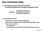

Other examples might come from robotics. For example, needing to compute a robot's answer to a human's question within the time expected for a response, or compute its best next motion before it falls off a cliff. Game-playing algorithms like chess would also fall in this category.
This comment was marked helpful 0 times.

TC scaling is useful when you're able to do things in an amount of time that matters to you. Most important time thresholds: interactive rates, over lunch break (i.e. come back after lunch and your results are ready for you), and overnight :)
This comment was marked helpful 0 times.

In the assignment 2 example, the time constraint is 30 FPS since anything less than that creates a visible stutter on the screen. So, for this type of scaling, we want to know how well more processors can do more work and render more complex scenes given the time constraint.
This comment was marked helpful 0 times.

For assignment 2, we don't want use our faster GPU to render more frames because the increase in frames-per-second is negligible to our eyes. By rendering more complex scenes instead, we get a more perceivable use for our faster GPU.
This comment was marked helpful 0 times.
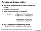

Memory-constrained scaling can be confused with the problem-constrained scaling, yet the memory-constrained scaling has "fixed amount of data per cell". So unlike problem-constrained scaling, as the number of processors increases the entire data size will increase, whereas in problem-constrained scaling, the size of the problem will remain fixed but the amount of data per cell will decrease.
This comment was marked helpful 0 times.
Memory-constrained scaling makes sure that each processor still receives the same amount of data to process as the number of processors is increased. However, depending on what operation you are processing the data with, the amount of work per processor could still change. As mentioned in this slide, matrix multiplication is a good example.
This comment was marked helpful 0 times.

Does this means that each thread on one core has a maximum of data processed per time unit due to how much memory the core has? So we have to find a way to parallel the program without increase the data store for each of the thread.
This comment was marked helpful 0 times.

@fangyihua, I think you're right, but to clarify, the limitation isn't just cpu-local memory, it's also the amount of main memory per core.
An example would be a condensed-matter physics simulation that needs statistical amounts of data: you want as big of a problem as you can get to improve the statistical properties of your results, so you make the data-set big enough to completely fill all available main memory.
This comment was marked helpful 0 times.

Just want to provide a note to distinguish different kinds of scaling here: First case: assign each frame to a machine (processor). Hence problem constrained as we did in homework 1. second case: given a fixed amount of time, try to create higher fidelity representation. Therefore time constrained. third case and last case: usually in order to deal with a lot of data (HD simulation in physics related fields), you can't handle the data set in one processor. Therefore assign the same amount of data to each processor and parallelize the simulation. Therefore it's memory constrained.
This comment was marked helpful 0 times.

How is element communicated in this example? Can someone help please?
This comment was marked helpful 0 times.

MC scaling: Since the memory usage per processor is fixed, we have the nice property that communication per computation decreases as both N and P increase. By looking at the previous slide, this becomes clear if we think about dividing the 2D grid ever more and sticking more dots inside each cell, and then imagining how much communication needs to occur as each of these increase. Essentially, each cell becomes more isolated in its work and so we see the best speedup.
This comment was marked helpful 0 times.

Communication overheads limits problem constrained scaling since as you break the grid into more subproblem, the number of grid blocks increases leading to a higher chance that an element will be on a block boundary.
This comment was marked helpful 0 times.

I am trying to understand how some of these values were computed. My understanding (for the time constrained scaling example) is:
Execution time is fixed at $O(n^3)$ by definition.
The total size of the grid $k \times k$ for some k
We need to calculate k. We assume that we will get a speedup linear in the amount of processors that we have, so we need $k^3/P$ to be $n^3$. This gives us that $k=nP^{1/3}$
Each processor is responsible for 1/P of the total grid. This is $k^2/P$ elements. Substituting the formula for k from step 3 we have that each processor is responsible for computing $n^2/P^{1/3}$ elements. This is the amount of memory that each processor will use.
Communication to computation ratio = elements communicated/ elements computed. Elements computed is $n^2/P^{1/3}$ from line 4. Elements communicated is $k/\sqrt{P}$ since k is the size of the whole grid. So the ratio is $(k/\sqrt{P})/(n^2/P^{1/3})$ $\ = k*P^{1/3}/n^2 \sqrt{P} $ $\ = nP^{1/3}P^{1/3}/n^2 \sqrt{P} $ $\ = P^{1/6}/n$
Question Why was n left out of the Big O for comm-to-comp ratio in TC scaling but included in MC scaling?
This comment was marked helpful 1 times.
I'm confused about the commu-to-comp ratio in MC scaling. computed element per processor should be NNP / P = N^2 communicated element per processor should be N*(P^1/2)/(P^1/2) = N And the ratio is N/N^2 = 1/N. Can someone help me out here?
This comment was marked helpful 0 times.
@martin: In my opinion, by definition, total work is (NP^1/2)^3 = (N^3)(P^3/2), so work for each processor is (N^3)(P^3/2)/P = (N^3)(P^1/2), so comm-to-comp should be N(N*P^1/2)/(N^3)(P^1/2) = 1/N
EDIT: @acappiello You are right, but comm-to-comp you compute should be (N^2)(P^1/2) / (N^3)(P^1/2) = 1/N, which is consistent with what @martin gets.
EDIT2: I corrected the mistake.
This comment was marked helpful 0 times.
@mschervi I believe that your analysis is totally correct. Since n is a constant, we can ignore it when writing the big O, but I'm not sure why there is a discrepancy.
@martin I'm having trouble with this too. Kayvon says that we're doing a lot more work, but communicating the exact same amount (video 46:00), which isn't totally true. We have more blocks in the grid as P increases, so communication goes up with P.
@xiaowend I don't think that's totally correct. Communication has to occur after each convergence iteration. So, the amount of communication over the entire program execution is "communication per iteration" x "number of iterations" which is $NP \times NP^{1/2}$. Total work is given by $(NP^{1/2})^3$, as you've said. So, I get a comm-to-comp of $(N^2P^{3/2})/(N^3P^{3/2}) = 1/(N)$.
EDIT: I don't think the above is still totally right. Thinking...
EDIT2: Made some changes to the calculation.
This comment was marked helpful 0 times.

Here is an argument for why the comm-to-comp ratio under MC scaling is constant. Note that the number of iterations is irrelevant for computing this ratio, because increasing iterations scales comm and comp by the same factor. As we MC scale, the size of the sub-grid seen by each processor remains constant. Thus the ratio between it's area (comp per iteration) and it's perimeter (comm per iteration) remains constant. Thus the comm-comp ratio is constant.
What is wrong with this argument?
This comment was marked helpful 0 times.


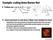
When considering TC/MC scaling, we should consider how different parameters are related to one another. In Barnes-Hut, the accuracy threshold ($\Theta$) and time step ($\Delta t$) should be scaled relative to n. These parameters contribute to the execution time of Barnes Hut which is given as $\frac{1}{\Theta^2 \Delta t} * n log n$.
(Resource: Parallel Computer Architecture, pg. 214)
This comment was marked helpful 0 times.
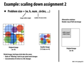
The obvious example here is if we just increased or decreased the dimensions of screen and then, for example, used a set like rand10k or rand100k. If we increased the dimensions of the screen, our problem might actually be easier (depending on our implementation) because the circles/tile would actually be much lower. Likewise, if we decreased the dimensions, we would have more circles/tile and this might make an implementation which divided the screen into smaller tiles work slower.
This comment was marked helpful 1 times.

This slide explains why we want to scale down the problem effectively by giving assignment 3 as an example where we have only limited number times to test our program on Blacklight due to long queue. Because of this limitation, we want to debug/test and make sure our code runs correctly in a small CPU machine before testing its performance in a bigger machine. Moreover, because it takes huge computational cost to diagnose the program as we experienced in assignment 2 where using printf costed severely to the performance, we do not want to debug and test on a full data set, but rather on a subset of data.
This comment was marked helpful 0 times.

The graph at the bottom of this slide -- cache miss rate vs cache size -- demonstrates a concept that is important for both programmers and hardware designers to keep in mind. Notice that the increase in miss rate as cache size decreases is discontinuous. These jumps in cache misses as the cache size decreases occur as the cache becomes too small to hold an entire working set of data (there are multiple jumps because there may be multiple critical working sets)
It's obvious that hardware designers building a system for a particular application will want to keep this in mind when considering the tradeoffs regarding cache-size, but it's also important for the programmer to consider how well his/her data is going to fit in the cache on the system they're programming for.
This comment was marked helpful 0 times.


Sometimes establishing the low watermarks is also useful, such as "Remove almost all math, but load same data" indicated in the the next slide. Running a program in a worst case scenario can give you an idea of how much improvement you actually achieved, and expose some of the limitations within the program.
This comment was marked helpful 0 times.

Sometimes "useless" instructions are optimized away by the compiler (like if we got some data but didn't do anything with it), which would limit one's ability to establish watermarks using these methods.
This comment was marked helpful 0 times.
@Arnie using the volatile keyword when defining your variables might help prevent compiler optimization. Additionally you can always use inline assembly.
This comment was marked helpful 0 times.
Some questions that were brought up during lecture were as follows:
What are my constraints? Is there a constraint on power budget/chip size?
What are the workloads that the processor will run?
What is "success"?
This comment was marked helpful 0 times.