@kayvonf, are the spikes we see attributed to thrashing like in virtual memory paging? Where the workspace is N+x but the size of the cache is N, therefore, every pass of the data pages things out to disk, and in this case evicts it from memory?
kayvonf
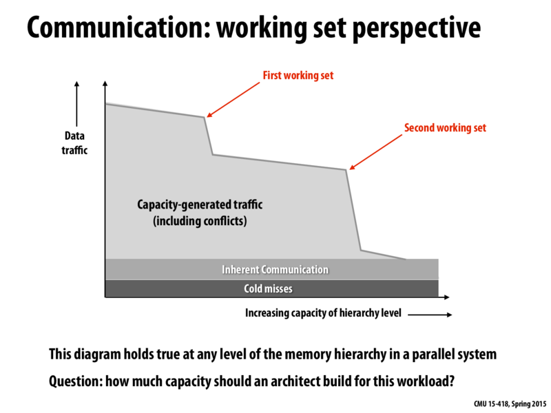
Virtual memory paging is moving data to disk when the total amount of allocated virtual memory exceeds the amount of physical memory in a machine. This graph is a plot of memory traffic as a function of cache size, not a plot of disk traffic as a function of main memory size.
Question: Who can explain this graph back at me? Even better, use the grid sample as an example.
Berry
The textbook was more concerned with stride - the 3rd dimension on this graph - but this graph says that as we increase the size of our cache our throughput grows smaller and smaller. Strangely enough it also seems like the textbook uses "size" of input rather than capacity of memory hierarchy level, which relates to whether or not we can fit our data into L1, L2, L3 or RAM. For this reason I am not sure how to elaborate this graph.
kayvonf
This graph says that for a given problem size, as the size of the cache is increased the number of misses goes down. Although describing the same idea, I suspect the experiment performed in the 213 graphs is different -- they are changing the size of the working set (changing the problem size).
Kapteyn
My attempt at answering the question:
The graph above illustrates the temporal locality of memory access patterns in most programs. The knees in the graph occur at the sizes of the first and second working sets because if the cache is large enough to hold the entire working set at once, we get a significant decrease in the number of conflicts that will occur as opposed to cache size increases before the critical point at the working set size.
To see why this is, we can use the grid solver example. Say we have an 8x6 grid G with 48 elements.
Our cache can only hold 16 grid elements at once and uses LRU policy. When we load the elements in the upper left 4x4 square of the grid, we can do convolutions for all of the elements in that square except for the rightmost column and bottom row of that square. Let's say the instructions are carried out such that blocks from the grid get loaded into the cache from left to right before moving on to the rows below.
Then when we want to perform convolutions on elements G[3,0], G[3,1], G[3,2], and G[3,3], we must reload 8 elements: G[3,0], G[3,1], G[3,2], G[3,3] and G[2,0], G[2,1], G[2,2], G[2,3] that we had already loaded before for the first square, because by that point they've been evicted from the cache.
If we were to increase our cache size such that it could hold 20 elements, then we can load 5x4 squares of elements instead, such that when we get to the rows below the first row of rectangles that get loaded into cache, we do not have to reload G[2,0], G[2,1], G[2,2], G[2,3], because the processor was able to compute convolutions for the elements G[3,0], G[3,1], G[3,2], G[3,3] when it loaded the first top left 5x4 rectangle due to the larger cache size, which accommodated elements G[4,0], G[4,1], G[4,2], and G[4,3].
If you draw out the overlapping blocks of the grid that get loaded in the case where we have a 16 element sized cache versus the 20 element sized cache, you'll see that with the 16 element sized cache, there will be 48 times when an element that's already been in the cache before, gets loaded into cache again. With the 20 element sized cache, there will be only 32 times when an element gets loaded into the cache again.
But this only saves us from loading 16 elements for ONE iteration over the grid. The grid solver will go over all elements of the grid in a while loop until the diff converges to zero. So since our cache uses LRU policy and we can't fit the entire grid in our cache at once, when we proceed to the next iteration of the while loop, we will have to reload the entire grid again, with all the additional reloads of elements that occur within one iteration of the while loop.
This slight benefit of 16 saved element loads per iteration corresponds to the gentle negative slope of the graph above before we hit the knee.
Now consider if we could load the entire grid, i.e. the entire working set into the cache at once. Now, we only have to load the elements in the grid once, for all iterations of the while loop. We will never have to reload anything. This significant save in data traffic corresponds to the knee in the above graph.
kayvonf
@Kapteyn: this was an outstanding answer. To summarize, you are pointing out how there are two important working sets in the solver example. One working set is a few rows of the grid. Another working set is the entire grid. As soon as a working set begins to fit in the cache, the number of capacity misses will drop sharply.
A good processor designer will understand the working sets of the world's most important programs, and then make design decisions that maximize bang-for-the-buck (where, in this case, bank for the buck is decrease in misses per increase in cache size).
Note to class: It's often helpful to summarize another student's post like I've done for @Kapteyn's post here. Saying the same thing in two different ways isn't a waste. In fact:
It's a great check to see if you really understand the post.
It's an opportunity to add a bit to the discussion.
Reading the same thing in two different ways is often a good way to learn something, so you're helping everyone else in the class. I often grab two textbooks when I'm trying to learn something new since equating the two explanations in my head is often helpful to check my understanding.
Look familiar? http://csapp.cs.cmu.edu/public/images/csapp2ecover-fullsize.jpg
@kayvonf, are the spikes we see attributed to thrashing like in virtual memory paging? Where the workspace is N+x but the size of the cache is N, therefore, every pass of the data pages things out to disk, and in this case evicts it from memory?
Virtual memory paging is moving data to disk when the total amount of allocated virtual memory exceeds the amount of physical memory in a machine. This graph is a plot of memory traffic as a function of cache size, not a plot of disk traffic as a function of main memory size.
Question: Who can explain this graph back at me? Even better, use the grid sample as an example.
The textbook was more concerned with stride - the 3rd dimension on this graph - but this graph says that as we increase the size of our cache our throughput grows smaller and smaller. Strangely enough it also seems like the textbook uses "size" of input rather than capacity of memory hierarchy level, which relates to whether or not we can fit our data into L1, L2, L3 or RAM. For this reason I am not sure how to elaborate this graph.
This graph says that for a given problem size, as the size of the cache is increased the number of misses goes down. Although describing the same idea, I suspect the experiment performed in the 213 graphs is different -- they are changing the size of the working set (changing the problem size).
My attempt at answering the question:
The graph above illustrates the temporal locality of memory access patterns in most programs. The knees in the graph occur at the sizes of the first and second working sets because if the cache is large enough to hold the entire working set at once, we get a significant decrease in the number of conflicts that will occur as opposed to cache size increases before the critical point at the working set size.
To see why this is, we can use the grid solver example. Say we have an 8x6 grid G with 48 elements.
Our cache can only hold 16 grid elements at once and uses LRU policy. When we load the elements in the upper left 4x4 square of the grid, we can do convolutions for all of the elements in that square except for the rightmost column and bottom row of that square. Let's say the instructions are carried out such that blocks from the grid get loaded into the cache from left to right before moving on to the rows below.
Then when we want to perform convolutions on elements G[3,0], G[3,1], G[3,2], and G[3,3], we must reload 8 elements: G[3,0], G[3,1], G[3,2], G[3,3] and G[2,0], G[2,1], G[2,2], G[2,3] that we had already loaded before for the first square, because by that point they've been evicted from the cache.
If we were to increase our cache size such that it could hold 20 elements, then we can load 5x4 squares of elements instead, such that when we get to the rows below the first row of rectangles that get loaded into cache, we do not have to reload G[2,0], G[2,1], G[2,2], G[2,3], because the processor was able to compute convolutions for the elements G[3,0], G[3,1], G[3,2], G[3,3] when it loaded the first top left 5x4 rectangle due to the larger cache size, which accommodated elements G[4,0], G[4,1], G[4,2], and G[4,3].
If you draw out the overlapping blocks of the grid that get loaded in the case where we have a 16 element sized cache versus the 20 element sized cache, you'll see that with the 16 element sized cache, there will be 48 times when an element that's already been in the cache before, gets loaded into cache again. With the 20 element sized cache, there will be only 32 times when an element gets loaded into the cache again.
But this only saves us from loading 16 elements for ONE iteration over the grid. The grid solver will go over all elements of the grid in a while loop until the diff converges to zero. So since our cache uses LRU policy and we can't fit the entire grid in our cache at once, when we proceed to the next iteration of the while loop, we will have to reload the entire grid again, with all the additional reloads of elements that occur within one iteration of the while loop.
This slight benefit of 16 saved element loads per iteration corresponds to the gentle negative slope of the graph above before we hit the knee.
Now consider if we could load the entire grid, i.e. the entire working set into the cache at once. Now, we only have to load the elements in the grid once, for all iterations of the while loop. We will never have to reload anything. This significant save in data traffic corresponds to the knee in the above graph.
@Kapteyn: this was an outstanding answer. To summarize, you are pointing out how there are two important working sets in the solver example. One working set is a few rows of the grid. Another working set is the entire grid. As soon as a working set begins to fit in the cache, the number of capacity misses will drop sharply.
A good processor designer will understand the working sets of the world's most important programs, and then make design decisions that maximize bang-for-the-buck (where, in this case, bank for the buck is decrease in misses per increase in cache size).
Note to class: It's often helpful to summarize another student's post like I've done for @Kapteyn's post here. Saying the same thing in two different ways isn't a waste. In fact: