


I was a little confused about Kayvon's question "How would you actually make the lists from this information?" Can somebody please summarize what was happening on this slide? Particularly transitioning from Step 2 to 3, and Step 3.
This comment was marked helpful 0 times.

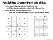
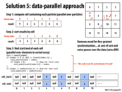
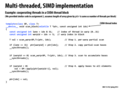
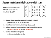
The transition from step 2 to step 3 takes place when the code block is run for each element of result (in parallel). This generates the two arrays that you see at the bottom. Then, we can generate a list for each of the cells using the cell_starts and cell_ends arrays. For the ith cell, our list is the elements of the result array from index cell_starts[i] (including this element) to cell_ends[i] (excluding this element). The reason we can just take contiguous portions of our result array as lists is because it's sorted by cell.
This comment was marked helpful 0 times.

We also need to keep the Particle Index array, right? For example we have for the 4th cell, cell_starts[4] and cell_ends[4] only includes the index 0 and 2, but the actual circle is 3 and 5, which is particle index[0] and particle index[1].
This comment was marked helpful 0 times.

@yanzhan2: correct, particle index array must be kept around. cell_starts and cell_ends refer to elements of particle index. For example, if we wanted to iterate over all particles in cell X:
for (int i=cell_starts[X]; i<cell_ends[X]; i++) {
    int index = particle_index[i];
    // do stuff ...
}
This comment was marked helpful 0 times.

In the step 2, there is a thread at every cell of sorted results. Every thread is responsible for checking whether there is a difference between the previous element and the current one. If there is one, it indicates the end of the previous list and the beginning of the current list. For example, for thread at result[2], it detects the end of 4s and the start of 6s. The special cases here are the first and last cell. Those positions are then written into cell_starts and cell_ends.
This comment was marked helpful 0 times.

LOL this was super helpful for the renderer lab :D
This comment was marked helpful 0 times.

@Yuyang, Yeah, I just watch this lecture today too! But I think we should modify it to make this work for Assignment 2. This method requires us to allocate a array with the length of number of particles. However, in A#2, we don't know the number of circles in advance. And we can't put such a huge array in shared memory to accelerate speed...We have to separate circles into groups.
This comment was marked helpful 0 times.

I'm curious if anyone was able to directly apply this method to Assignment 2 (are we allowed to discuss homework solutions here?)
It seems that the main difference between the application in this slide and the circle renderer is that circles can lie in multiple cells. While I see how related data-parallel methods can be applied to circle render (what my partner and I did), it's unclear to me how these precise steps can be followed.
This comment was marked helpful 0 times.

@jon I did it this way for Assignment 2. If you just assume the worst case, that all circles cover all cells, then you can allocate memory accordingly. The cell size then needs to be chosen to not run out of memory in that worst case. I looped over all of the cells covered by a circle and added them to a global list like in this example.
The thing that surprised me a bit was that while this step might seem like it would be slow because of global memory accesses, atomics, and each circle causing different branching paths, in fact it was quite fast compared to the sorting step. The sort was by far the slowest part of my renderer, even though I was using Thrust's very fast parallel radix sort.
This comment was marked helpful 0 times.

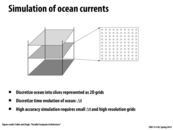

How are the interactions dealt with between levels? This seems like a 3d problem, we somehow simplified it to 2d. Does the algorithm simply access points from other 2d grids to find there interaction with the current grid?
This comment was marked helpful 0 times.
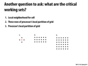

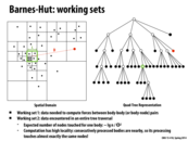
So, the advantage in the second arrangement is that the third row is already there in the cache when you want to store the information, so there would be fewer cache misses.
The optimization in the third arrangement is that almost all the information is there for you, so there are almost no cache misses except for the cold misses.
Is there any advantage to the first arrangement?
This comment was marked helpful 0 times.

I think the three working sets mentioned here are just different amounts of caching that can be done. What you pointed out about the second and third arrangement are correct, but in situations where there are cache size limitations, we would have to go with the first arrangement, which is advantageous when using a small cache because the values needed to calculate for that particular cell are loaded into the cache.
This comment was marked helpful 0 times.

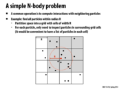
I agree with @mpile13; I don't see any benefit to being able to fit the first set into your cache. To update the red dot, you only need to access each of the black dots once, so having them in your cache doesn't help any. Having data in your cache is only helpful when you're accessing it repeatedly.
This comment was marked helpful 0 times.

Caches typically bring in data in block amounts, which means if the block size was large enough we could access various elements around the grid such that it eventually pulls in something like the smallest working set for a cell.
This comment was marked helpful 0 times.

@sbly You mean there is not much benefit to caching /just/ the first set? Even though the black dots are only used once when updating the red dot, they are used other times to update other dots in the current part of the partition.
This comment was marked helpful 0 times.

I believe that the benefit to being able to fit the first set into your cache is that given the limitation that your cache can only fit 5 points (unlikely, but this is for hypothetical purposes), it is possible to arrange your data such that with one cold miss, all the data necessary for a single computation can be loaded.
However, given some other arrangement of the data, perhaps in row-major order, loading all the data necessary for a single computation might take 3 cache misses. This is important if the computation for each point is done in a different thread. In this case, each thread will not utilize the extra points in the cache, and there will be wasted memory bandwidth and cache space.
This comment was marked helpful 0 times.

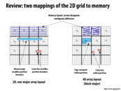

Why is the layout on the right considered 4D? If the block is the third dimension, what's the fourth?
This comment was marked helpful 0 times.

Each block is two dimensions, not one. You could declare an array like on the right as so: Array[num_blocks_y][num_blocks_x][block_size_y][block_size_x]. A 3D array would only have one 'row' per block whereas this array has multiple introducing a 4th dimension.
This comment was marked helpful 5 times.

in the 4D array layout, the cache line (in pink) is shown to span 2 rows. Is there a way to actually implement a data structure such that the processor loads a cache line in such a manner?
This comment was marked helpful 0 times.

@sss I think you would represent the 4D array using a single 1D array such that the contiguous addresses follow the direction of the arrows shown in the picture. This would be similar to the same manner that you often represent 2D images in a 1D format.
Say that we have an array that is 2-blocks wide, 1 block high, and each block has 2 elements along the x axis and 2 along the y. Let B(a,b) be the block at index (a,b) and E(x,y) be the element in a block with coordinates (x,y) (where I'm indexing y to go from top to bottom, x from left to right, and same with a and b).
Then, in memory, we can lay it out as follows:
------------------|-----------------|-----------------|-----------------|
| B(0,0) | B(0,0) | B(0,0) | B(0,0) | B(1,0) | B(1,0) | B(1,0) | B(1,0) |
| E(0,0) | E(1,0) | E(0,1) | E(1,1) | E(0,0) | E(1,0) | E(0,1) | E(1,1) |
------------------|-----------------|-----------------|-----------------|
So, visually, the cache line would span 2 rows, but in actual memory, it wouldn't.
As you can imagine, indexing into this array is lots of fun, so let me know if I made a mistake :)
Specifically, if element at the start of the cacheline is at index block_idx_x, block_idx_y, x, y (where block_idx_x, block_idx_y are the x and y indices of the block, x, y are the coordinates of the element within the block, where y is really the row), then you can access it as
Array[((block_idx_y * num_blocks_x + block_idx_x) * (block_size_x * block_size_y)) + (y*block_size_x + x)]
Let's break this down....
When I index into this array, I like to think of starting at the upper left of the array and counting the number of elements I have to go through as I follow the arrows (from the picture).
First I want to know the number of blocks that I skip over to get to my block. This should be the number of rows I go through * number of blocks/row + the horizontal index of my block:
(block_idx_y * num_blocks_x + block_idx_x)
Then if I multiply this by the number of elements in a block, I get the number of elements I skip through:
(block_idx_y * num_blocks_x + block_idx_x - 1) * (block_size_x * block_size_y)
This should put me at the start of my block. Finally I just need to find the element within the block:
(y*block_size_x + x)
This comment was marked helpful 0 times.


I don't understand how 4D block assignment achieved faster runtime overall. Would someone explain it to me?
This comment was marked helpful 0 times.
From what I understood, if you look on the previous slide, the diagram on the left shows that you organize your data in row-major order in memory (i.e. (row,col): [(0,0), (0,1), (0,2)...] ). Thus, if you tell your 16 different processors to divide up work by blocks, you will have a lot more cache misses since cache lines could be stored across the partitions/processors. However, on the right side (of previous slide) if you store your data in block-major order (i.e. (row,col): [(0,0), (0,1)..(0,5),(1,0),(1,1)...]), now the data is laid out in memory by how the processors work on it. You will now have less cache misses and more importantly less sharing between the processors, so they can work independently on their own data.
This comment was marked helpful 0 times.

With the 4D block arrangement, there's now at most 2 cache lines that can be shared per block. With the row-major layout, there are up to 2*(block height) cache lines that could potentially leak across blocks.
This comment was marked helpful 0 times.

A 4D block arrangement prevents cache misses, because the data is arranged in memory in blocks corresponding to the processors, like @selena731 said. However, faster runtime is mostly achieved by reducing sharing between blocks. This prevents cache coherence misses (that might occur due to the ping-pong-ing between processors of data) because the processors are sharing fewer lines, as @kkz mentioned.
This comment was marked helpful 0 times.


I found a good site that thoroughly explains the Barnes-hut algorithm, so if you want to understand the algorithm, and consequently, the optimizations from parallelism better, its a good read.
http://arborjs.org/docs/barnes-hut
This comment was marked helpful 0 times.
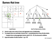

I think this construction is very clever, and I think a lot of other problems could take advantage of a similar setup. For example, suppose one wanted to simulate the transmission of a pathogen within some host population. The distribution of hosts could be used to build a contact hierarchy, and the probability that any infected host exposes any susceptible host to the pathogen could be found efficiently by walking though the tree. This would be much better than the naive approach of iterating over all pairs of hosts to check for transmission events.
This comment was marked helpful 0 times.

Is there a way to dynamically maintain the tree structure for reducing cost (like adaptive Huffman coding)?
This comment was marked helpful 0 times.

I don't think there is a way to dynamically maintain the tree other than generating the quad-tree from the locations of the particles in the simulation. The tree needs to represent which particles are close to each other, so that is the tree structure.
This comment was marked helpful 0 times.


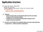
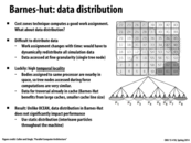
Wouldn't calculating the local per-body counters not be cheap to compute? The increment operation would have to be atomic so that the count is accurate, just like computing the number of nodes in the frontier in assignment 3. If the operation is atomic and many bodies are accessing the same counter, there will be major contention there which would increase the time of computation.
This comment was marked helpful 0 times.
Because the counters are per-body, and we parallelize this algorithm per-body, the counter would not require any atomic operations and would be local to each thread.
This comment was marked helpful 0 times.

Question: I'm not sure I understand how the work division for the tree on this slide is found. If each processor simply does an independent depth first search until it reaches W/P work completed, then how are we sure there won't be any overlap in the assignment of bodies computed by the processors?
This comment was marked helpful 0 times.

Each processor performs DFS and accumulates a list of work seen so far. Thus, we can have processor i do the particles that correspond to the items in the list from [iW/P,(i+1)W/P), so it does up until the last particle that it sees below the upper work bound. Then, the next processor will carry on at the next particle (the first particle that makes the list have at least (i+1)W/P work), and there will be no overlap.
This comment was marked helpful 0 times.

I'm somewhat confused about how W is found for this algorithm. How can we estimate how much work each body will take to compute, without actually doing the computation? Is this what is referred to on the previous slide, when it says "for each time step, for each body, record number of interactions with other bodies"? If so, it also says this is cheap to compute, however looking at slide 27 it seems as if doing this computation increases the "busy" time by a significant amount. However, since it does decrease the overall time, it seems like it is worth it.
This comment was marked helpful 0 times.

Each processor perform one DFS and accumulates a list of work. I think this would be slower than having one processor performing the DFS and partition the work and assign different partitions to different processors. I'm confused about the parallelism here.
This comment was marked helpful 0 times.

@paraU I think it depends on how W is computed. I think you can compute W so that each node in this tree knows how much work is needed to process all of its children. That way, the DFS on this tree doesn't need to visit all of the nodes. As a concrete example, let's say that the root node will require W, and each of the four children of the root will require W/4. Then processor 8 in this example can skip the traversal of the left-most child, since processor 8 needs to handle the list [7W/8, W), and the left-most child contains the list [0, W/4). The idea is similar to alpha-beta pruning.
But even if W wasn't computed this way, one processor assigning work will require some amount of synchronization (the other processors need to wait and then receive their assignment).
This comment was marked helpful 0 times.
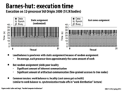

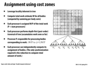
As mentioned on the previous few slides, the "cost-zone assignment" increases locality, and reduces the overall execution time compared to static assignment.
However, it is interesting to note: computing this processor workload distribution has a cost. As you can see in the graphs above, the "busy" section of the graphs is higher on the "cost-zone assignment" implementation than on the "static random assignment" implementation.
Moral of the story? Doing more work to preserve locality and maintain a balanced workload still has the potential to decrease overall computation time.
This comment was marked helpful 0 times.
Looking at the complexity of writing code for the extra assignment computation, and only 5s of increase in time (compared to the total 30s), is this really worth it? Can we really argue that the right hand side approach uses the resources better?
This comment was marked helpful 0 times.
@selena731: I guess it just matters how much performance you want to squeeze out, and how willing you are to obtain it. The more advanced assignment scheme improves performance by about 15% over random assignment.
This comment was marked helpful 0 times.

Programming to eliminate bandwidth problems seems to be programming to the hardware. If I were on a machine with a tiny cache, the speed up from attempting to find locality may not be worth it, right? In places where multiple types of machines and hardware are used, I'd imagine there is a bit of a tradeoff that needs to be considered.
This comment was marked helpful 0 times.

This is a really interesting example as it correctly shows that sometimes doing extra work for assignment or balancing might lead to over all higher speedups.
This comment was marked helpful 0 times.


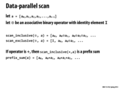


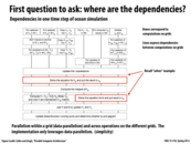
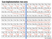
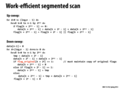
We concluded in lecture that the constant for the work was around 3 and the constant for the span was 2.
This comment was marked helpful 0 times.


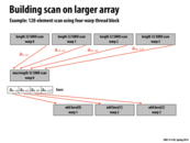

It seems to me that the base of the rightmost arrow should be pointing to the other cell of the base (a_{0-95}), if anyone is keeping score.
This comment was marked helpful 0 times.
@tcz: We do keep score. You are correct. A_{0-95} should be pointing to the "add base[2]" box. I'll fix this shortly.
This comment was marked helpful 0 times.
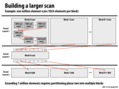
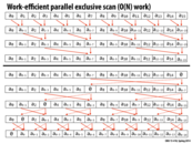
Question: It does seem like if N is super big, we would have to split the scan into a few more scans in the second step, therefore leading to some more 'result combining' and thus longer span (in the middle block). However the extra number of 'result combining' we do is just logarithmic of N, so would that be an example of a very 'scalable system'?
This comment was marked helpful 0 times.
@Yuyang. Correct. The span is log N, so as N gets bigger span of the computation is going to increase.
This comment was marked helpful 1 times.


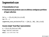
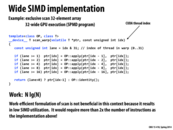
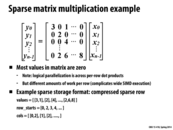
I'm confused. Wouldn't we just scan each of the arrays separately in parallel? This is real easy to do if it's stored as a two-dimensional array. Why do we use this "head-flag" representation?
This comment was marked helpful 0 times.
@sbly: Thought experiment: What if array 1 was one million elements, and array two was 10 elements.
This comment was marked helpful 0 times.

Could someone elaborate one Kayvon's thought experiment? The work being done on array1 is much more costly than on array 2, but there's no way getting around that. Is it just that the head flag indicates where the partition is being made which can then later be used to call scan on each of the arrays separately?
This comment was marked helpful 0 times.
I interpretted @sbly's suggestion as: if we have N subarrays, just parallelize over the subarrays (yielding N independent pieces of work). I presume that each sort would be carried out sequentially.
So in the case of N=2, imagine if one of those subarrays was huge, and the other tiny. What problems do you see with the parallelization scheme I just described?
This comment was marked helpful 0 times.

The problem with the given parallelization scheme is that simply splitting up the tasks into N different tasks does not account for workload imbalance, and that the performance gains that we can gain through parallelism would be diminished.
This is the same problem that we were presented with in the Prog 1 Mandlebrot of Asst. 1.
This comment was marked helpful 0 times.

Is it correct to say that this approach is useful only because we have the "head-flag" representation? Suppose we have a list of lists but do not know where they are in the original data, this will not work? I.e. we have a[] and maybe data[], but do not have flag[].
This comment was marked helpful 0 times.


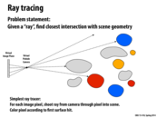

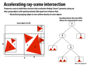
In most implementations, how does the distance between the virtual pinhole and the virtual image plane affect the image? In photography, it would put objects at different distances from the camera in focus. To get this kind of focusing effect in ray tracing would there need to be some math done to adjust how rays interact with the edges of objects at different distances?
This comment was marked helpful 0 times.

I would imagine that it would affect things such as what is actually seen (for example, none of the yellow/gold circles above would be rendered because they are not visible from the pinhole), brightness of pixels corresponding to circles at varying distances, and other such features. I think your right, there would be math done, and probably to best replicate real life, like your photography example.
This comment was marked helpful 0 times.

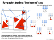
Some edge effects in ray tracing (e.g. having a smooth instead of jagged edge) can be simulated by taking a large number of samples per pixel. Different samples originating from the same pixel would present an even better case for rays in a packet than rays from adjacent pixels, since locality would be expected to be even better.
This comment was marked helpful 0 times.
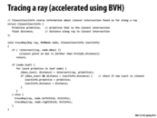
traceRay is a recursive function that computes the closest intersection of the ray ray with the scene geometry contained within the sub-tree rooted by node. As the ray is traced through the subtree, the struct isect maintains information about the closest intersection found so far. This information consists of the distance along the ray to the closest intersection, and a reference to the scene primitive that yielded this intersection.
traceRay works as follows:
It first determines if the ray intersects the bounding box of
node. If it does not intersect the bounding box, or if an intersection does exist, but is strictly farther than an intersection found so far, then he function returns. This "early out" is valid because it is not possible for any geometry insidenodeto generate a closer intersection.If the node is an interior node,
traceRaythen recurses on the nodes for the two children.If the node is a leaf node,
traceRaychecks for intersections between the ray and each primitive in the leaf (see call tointersect()function). If an intersection exists and that intersection is the closest scene intersection found so far, this information is stored inisect.
To give you a sense of how traceRay is used to make a picture, the overall basic structure of a ray tracer is given below. Notice how iterations of the outermost loop are independent and can be performed in parallel.
BVHNode root;

for each pixel p in image:  // iterations of this loop are independent
   Ray r = createRay(p)     // r is a ray traveling from the image pixel
                            // through the camera's pinhole aperture
   ClosestIectInfo isect;
   traceRay(r, root, isect);
   if (isect indicates a hit)
      color p according to isect.primitive;
This comment was marked helpful 0 times.

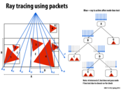
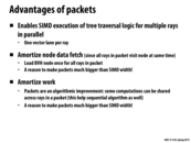

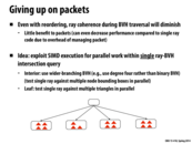
This seems like a reasonable idea, but it also seems that taking advantage of SIMD in this way is almost not worth it... unless the packet size is many times larger than the processor size. Sure, in this example we save 1 SIMD instruction to work on 7 of 8 instead of 7 of 16, but I imagine if there were say, 2 of 16 rays, there would still be a lot of wasted resources. At least having a larger packet size would allow for the cases where, say 4 of 64 can be compressed to 4 of 8, or something like that.
This comment was marked helpful 0 times.


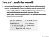
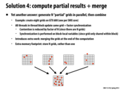
An important observation is that Solution 1 duplicates computation in order to reduce synchronization. (It completely eliminates synchronization in this case). Solutions three and four trade off memory footprint (they duplicate structures) in exchange for reducing contention. A similar idea was used to reduce synchronization in slide 38 of Lecture 4, when we reduced three barriers to one in the solver example.
Question: When might it be a bad idea to trade off memory footprint for synchronization/contention?
This comment was marked helpful 0 times.
Trading off memory footprint to reduce contention is not worth it if the extra steps required (in this example, the merge) take more time than the time we saved through better synchronization. Another more obvious example is if we would have to allocate a lot of memory or don't have enough memory to do so. Thinking of NUMA, accessing that memory might also take considerably longer as we get further away.
This comment was marked helpful 0 times.
The idea of "not having enough memory" barely even exists anymore, at least on CPUs; there's significantly less memory on GPUs so maybe there you'd care more?
Probably more of a problem is if this memory tradeoff significantly increases the bandwidth of memory accesses: if the extra memory usage means a lot of extra read-writes that aren't cached, it will significantly hurt performance, possibly worse than the gain from synchronization or contention.
This comment was marked helpful 0 times.