


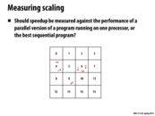

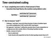
On the one hand, if we measure the speedup against a parallel version running on one processor, we can measure the scalability of our algorithm as we increase the input size and the number of processors. Doing it this way would allow us to make judgments about how our algorithm itself scales. However, if we want to measure how useful our algorithm is compared to running sequential code, or how "worth it" it is to parallelize the code, we should measure speedup against the best sequential program, because in the real world the choice is not between a parallel program on one processor and a parallel program on multiple processors. The choice is between a parallel program on many processors and an optimized sequential program on one processor.
This comment was marked helpful 0 times.

I would agree that the "best sequential program" should be the real measuring stick. Often, the parallel version of a program running on one processor has a lot of overhead, such as creating elaborate data structures (such as the data parallel particle simulation from lecture 8. The parallel version is usually optimized to work well only when given many workers.
So, it's pretty unfair to compare the "best" parallel program to a possibly terrible sequential program (though it probably makes for nicer graphs.)
This comment was marked helpful 0 times.

As @jon and @jmnash said, I also think speedup should be measured against the best sequential program. If we want to see the speedup obtained by parallelizing the code, rather than the speedup obtained by adding more processors, we should compare against the sequential version. There can be a lot of overhead involved in the parallel version, even if we're only using one processor. Also I think this approach is better because it is unlikely we will run the parallel version on one processor. However, if we want to measure how our algorithm scales when we add more processors, comparing it against the parallel algorithm on one core seems reasonable.
This comment was marked helpful 0 times.


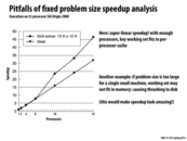
Just to make sure - the reason why the ocean simulation speedup actually decreases after ~16 processors is due to the communication costs increasing enough for it to overwhelm any speedup in computation (i.e. the communication-to-computation ratio is large because the size of the simulation is small and the number of processors is large). Am I explaining this correctly?
This comment was marked helpful 0 times.

Correct. The overhead of communication grows as processor count increases. After 16 processors the extra cost of this overhead overcomes the benefits of additional parallel execution. This is the reason we observed a slowdown between 16 and 32 processors.
This comment was marked helpful 0 times.
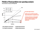

The communication-to-computation ratio is saturated more quickly as processors are added and as the size of the problem instance decreases. To take advantage of more processors it may be necessary to increase the size of the problem instance, which, depending on the problem, might not be a trivial task. Benchmarking, as in the chart on this slide, can help determine what the best instance size and number of processors is for any given problem. In this case, the best speedup (~24x) is achieved with 32 processors on a large instance of the problem.
This comment was marked helpful 0 times.

Interesting quote from lecture which summarizes this slide really well --
"We aren't just adding more processors, we are adding more cache memory".
In between 8 - 16 processors, the working set of the grid solver fits within cache memory of each processor. This minimizes the number of cache misses, and these misses all happen in parallel. By avoiding these memory misses, we get "superlinear" speedup.
This comment was marked helpful 1 times.

Because the working set of the grid solver fits within the cache memory, the number of cache misses is minimized. However, for this to occur the data must have excellent spatial locality in the cache such that it's all excellently packed and accessed so that we don't need to retrieve from the cache often. This situation is a rare occurrence which is why super-linear, while possible, is pretty rare as well.
This comment was marked helpful 0 times.


I was looking up scaling online, and i came across this post that talks about the difficulty of truly assessing parallel efficiency plotted on a log-log scaling, which seems to be more common. Are most of the plots in this course done on a log-log scaling as well or linear scaling? The link below shows some valid benefits of both attempts and why people would use one over the other to analyse or showcase results.
When making our final project, should we also choose a plotting that is more beneficial to our aims or stick to a standard plotting for all groups?
http://scicomp.stackexchange.com/questions/5573/log-log-parallel-scaling-efficiency-plots
This comment was marked helpful 0 times.
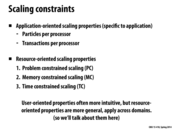

What's an example of a user-oriented property?
This comment was marked helpful 0 times.

Taken from the textbook for the course, user oriented properties are things like number of rows of a matrix per processor, number of I/O operations per processor, etc, in addition to the things listed under application oriented properties (maybe it's just another name for it?). I supposed it is named as such because as a user it is "easy" to follow constraints such as keeping the number of X per resource.
This comment was marked helpful 0 times.

The slide seems to be implying that user-oriented properties and application-oriented properties are the same thing. I think this makes sense since, to the person who's developing a computing platform (in this lecture, a processor), programmers are users. They think of scaling in terms of how their problem breaks into subproblems, while you (the processor developer) think of scaling in terms of the performance of your system.
This comment was marked helpful 0 times.
@bxb There's a textbook for the course?
This comment was marked helpful 0 times.


Why divide up the metrics instead of just using one? This one seems to generalize to include the information of the others.
This comment was marked helpful 0 times.

If you're talking about how we calculate speedup, it appears that the other metrics are indeed the same as this one, with either fixed time or fixed work. I think the reason they're separate metrics is to only include the variables that matter--they're just simpler versions of this equation.
This comment was marked helpful 0 times.
@bwasti: I don't think I see the generalization you're talking about. Could you explain in more detail why this metric has the information of both the other two?
This comment was marked helpful 0 times.


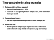
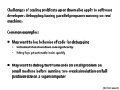
Why is it that the animation complexity is bounded by the memory on each machine? Are the communication costs too large to distribute it across multiple machines?
This comment was marked helpful 0 times.

If an animator wants to see motion in real time, yes. It depends on how long a delay you want between specifying the animation, rendering, and output.
This comment was marked helpful 0 times.

I believe the animation complexity is bounded by the memory on all the machines. The processing is distributed across all the machines, but the maximum number of polygons that can be rendered is still bounded by the total memory available on all the farm machines.
This comment was marked helpful 0 times.

Im confused about what the last bullet point is saying, specifically what the footprint refers to. Does this mean that the total memory of the system is constrained but if you add more processors, there has to be more memory allocated to managing processor interactions?
This comment was marked helpful 0 times.

@vrkrishn I'm thinking the same thing as you are. I believe that in general, the more processors you are using, the more overhead there is to manage them. One naive example that I can imagine (which I might be completely wrong about) is that if we're rendering a scene, and we want it raytraced (a common option in final renders), then splitting the scene into layers will require that each processor have information about the above and below layers in order to carry out its own computation. In that case, keeping that information handy can create this memory overhead, as rendering sequentially can just keep all the memory in one place.
This comment was marked helpful 0 times.


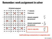
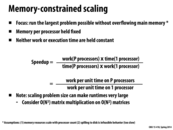
Why is comm to comp ration $O(P^{0.5})$ instead of $O(P^{0.5}/N)$? The ratio is just elements communicated divided by elements computed right?
This comment was marked helpful 0 times.
Your understanding is correct, but in this slide we're talking about how communication-to-computation ratio scales as the number of processors P increases. So the slide treats N as a constant and only gives scaling as a function of P.
This comment was marked helpful 0 times.


I am a little bit confused about above Time-constraint scaling example.
Why scaling the grid size to be k * k would result in speedup k^3/p?
This comment was marked helpful 0 times.
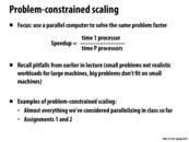
Time-constrained scaling means that as more processors are used the problem size is also increased so that the overall runtime stays the same. We know the problem takes $O(N^3)$ time on one processor, so when working on a larger grid with P processors, we need to select a grid size $k$ such that $k^3/p = n^3$. (This assumes that the P-processor version of the code perfectly uses the P processors... e.g., gets perfect speedup)
This comment was marked helpful 0 times.

I believe that the Comm-to-comp ratio should be computed not as (elements computed per process) / (elements communicated per process), because elements computed per process is not the same as (less than) the work done in each process. In this example, in general if we have a potentially scaled up grid of k by k elements, every processor works with b = O(k^2 / p) elements and takes t = O(k) while communicating c = O(k / sqrt(p)) elements. CtCR should be c / (b * t) = O(sqrt(p) / (k^2)). In the case of Problem-constrained scaling, we have k = n, which gives us CtCR = O(sqrt(p) / (n^2)). In the case of Time-constrained scaling, we have k = n * p^(1/3), which gives us CtCR = O(1 / (n^2 * p^(1 / 6))). In the Memory-constrained scaling case, we have k = O(n * sqrt(p)), and CtCR = O(1 / (n^2 * p^(1 / 2))). If we treat n as a constant, we have O(sqrt(p)), O(p^(-1 / 6)) and O(p^(-1 / 2)) as the respective CtCR's for this example.
This comment was marked helpful 0 times.


So not quite analogous to PIN, but Nvidia does offer a profiler to run at the same time as your CUDA programs to give you perspective on how well the GPU is being utilized. It looks like OS X's Activity Monitor on steroids. The Analysis and Timeline views look like they could be enormously useful in the future (and would have been a huge help on Assignment 2.) nvprof is runnable from ghc machines, although I couldn't get the program to launch over SSH. If anyone has success with it, do share! See here the console output of running
nvprof ./render -r cuda rgb on the gates machines:
==4775== Profiling application: ./render -r cuda rgb
==4775== Profiling result:
Time(%)      Time     Calls       Avg       Min       Max  Name
 88.50%  14.425ms         8  1.8031ms  1.6160ms  2.7931ms  [CUDA memcpy DtoH]
  9.17%  1.4951ms         7  213.58us  213.31us  214.05us  kernelRenderPixels(void)
  2.27%  370.31us         7  52.900us  52.704us  53.376us  kernelClearImage(float, float, float, float)
  0.06%  9.3440us         9  1.0380us  1.0240us  1.1520us  [CUDA memcpy HtoD]


This comment was marked helpful 1 times.

And in case anyone was wondering, to get the visual version of the profiler as pictured, run nvvp over an X session.
This comment was marked helpful 1 times.
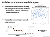
Explanation of Pareto curve: See that graph in the top right? The left axis is essentially "How expensive is each operation, in terms of power?". The right axis is essentially "How many operations are we trying to run in a small amount of time and space?"
The "Pareto curve" is the curve along the bottom right -- it minimizes energy usage, and maximizes performance + density. Each of the blue dots could represent a different chip design, and the chips in the bottom right would provide the best benefits with the lowest cost (where cost is measured in terms of nanojoules per operation).
This comment was marked helpful 0 times.

Also interesting to think about here: the Pareto distribution (note that the name in the slides has a typo) isn't specific to GPU performance but actually a probability distribution which can be used to model a wide variety of phenomena.
It seems like the Pareto curve referenced in the slides is actually a backwards Pareto distribution.
This comment was marked helpful 1 times.

For the cache size and miss rate curve, different benchmarks would have different working sets. So should the curve be the average of some benchmarks?
This comment was marked helpful 0 times.
@yanzhan2. Absolutely, the curve is dependent on the workload. So in designing and architecture it would be wise to consider average-case performance over a collection of important workloads.
This comment was marked helpful 0 times.
@wcrichto Ah I was wondering about that, I thought the names were just really similar. Do you know why this is called the Pareto curve? The fact that it looks like a backwards Pareto distribution just seems like a coincidence with this particular example. Is there any mathematical reason why these curves look like backwards Pareto distributions?
This comment was marked helpful 0 times.

@sbly @wcrichto
It is apparently because this economist Pareto guy has two major contributions:
One is the beloved Pareto distribution :D the other is Pareto Optimality.
This comment was marked helpful 0 times.


Just to clarify:
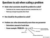
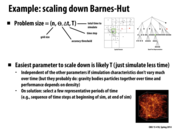
These need to be preserved when changing the per-instance problem parameters (for example: In the N-Body simulation: time simulated, where bodies are, the approximation distance). If the items in the slide are not preserved, then the scaling measurements are not valid.
am I right?
Edit: Ah, going forward in the slide deck, I see that scaling down the problem while preserving these properties allows measurements to be done which accurately reflect how a larger problem will behave.
This comment was marked helpful 0 times.
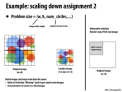

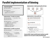
Question: on the bottom left, two issues with scaling the entire image down are mentioned - the ratio of 'filtering' to per-pixel work changes, and the concentration of circles in a tile changes. But when you use just a quarter of the image as shown on the right, aren't both of these true as well?
This comment was marked helpful 0 times.
bstan. The concentration of circles in a tile stays unchanged since we're rendering the same tiles, just not all of them.
The ratio of circle filtering work to pixel work does not change in one possible implementation of the renderer (the one I was envisioning when I made the slide), and thus this scheduling down strategy is a sound one. But I could see this ratio changing in other implementations -- so yes, there was a bit of unclear thinking on my part. This reinforces the point that one must think carefully about how a program works to determine if a scaling up or down strategy changes key performance characteristics.
This comment was marked helpful 0 times.
Let me check my understanding here: the one on the left changes the work done per-circle, so if your renderer parallelizes along circles then scaling the image down is bad. On the other hand, it also changes the amount of work done binning circles since they're in significantly fewer bins, so if you're parallelizing along pixels the left approach is also likely bad. The approach on the right leaves circles the same size so they take the same amount of time to process, and also fall into the same bins, so it's likely to be a good method of scaling for the two renderer approaches I just mentioned. Can anyone tell me what renderers would struggle on the second scaling method, but not the first?
This comment was marked helpful 0 times.

I don't think that there the second scaling method (right hand side) would ever be worse than the first scaling method, since we are simply removing data that needs to be computed, and communication overhead is the same or lower as the number of tiles is the same too.
This comment was marked helpful 0 times.


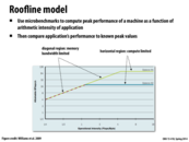
The diagonal region implies that we can continue to add instructions and get higher because rate to get more data is slower than the rate to compute.
Also, the graph suggests that it is harder to use Opteron X4 machine efficiently because we need to give more data.
This comment was marked helpful 0 times.

Did this test take advantage of memory pre-fetching? (Assuming that arithmetic data was pulled from RAM).
This comment was marked helpful 0 times.
This graph also seems to indicate that the Opteron x4 has a faster memory bus
This comment was marked helpful 0 times.

@Q_Q This actually does not show the Opteron x4 has a faster memory bus. This is showing that they have the same one. Note that when they are both bandwidth limited (the sloping portion of the graph), they are getting the same performance. As soon as the Opteron x2 is compute limited the Opteron x4 has better performance as it has more processing power.
This comment was marked helpful 0 times.
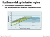

So by adding ILP/SIMD, in the range between 1/2 to 2 on the x-axis, the limitation which used to be on computation becomes a bandwidth limitation?
This comment was marked helpful 0 times.
The program without SIMD/ILP optimizations ("TLP only") is bandwidth limited (assuming "unit stride accesses only" until the operational intensity hits 1/2 flops/byte. By increasingly compute throughout via SIMD/ILP optimizations, the program becomes bandwidth limited at 2 flops/byte.
This comment was marked helpful 0 times.

Sometimes it is also important to realize that doing something like changing all array accesses to A[0] could consequently result in more/less work somewhere else in the code, which could really skew the watermarks that you get and really take away its value.
This comment was marked helpful 0 times.
@ycp. Absolutely, so you'll need to be careful. Another issue to watch out for is that modifying the code can cause certain compiler optimizations to kick in. For example, if you modify the program to load values and never meaningfully use them ("take out math"), dead code elimination during compilation might kick in an remove the read from the program entirely!
This comment was marked helpful 1 times.
Is there any good way of knowing when a compiler will eliminate dead code, besides of course looking at a dump of the assembly? I assume doing something like a = 1+2; and never using 'a' would get eliminated, but if i do a = ..., b = a+..., c = a+b, can the compiler detect that you don't need the entire chain of dependent variables?
This comment was marked helpful 0 times.

There is a special dead code analysis that compilers run in order to determine whether something can be eliminated. The statements you have described, assuming a, b and c are ints, could be constant folded and propagated away by a compiler and consequently, eliminated as dead code if they are not used elsewhere. If you do funky things with memory accesses however, the compiler might be a bit more conservative about it.
This comment was marked helpful 0 times.

To add to what @rokhinip said, I've found the dead code eliminator to be pretty hard to avoid (even with weird memory accesses and things) without potentially losing other optimizations you might want to keep (declaring values as volatile, for example). The easiest way to measure memory access time would probably be to add timing code around memory accesses, and leave the math do be done afterwards.
This comment was marked helpful 0 times.
Is there any good methods to see if the performance problem is due to memory bandwidth bound?
This comment was marked helpful 0 times.

@analysiser: looks like the "remove all math..." bullet point partially addresses this... @jhhardin: That sounds like it would work well if most of the memory accesses are bunched up, as are the chunks of computation. Are there good utilities for generating statistics like those we saw in previous lectures? (e.g. graphs of bus traffic/cache misses/etc)
This comment was marked helpful 0 times.
The two main answers people gave in class were "what will the processor be used for?" (what types of applications/which are the highest priority/etc) and "what resources do I have to work with?" (both logistically in terms of the design, and also in terms of the processor - is it limited in how much power it can have? how much memory it can have? how physically large it can be?)
This comment was marked helpful 0 times.